This page summarizes the process of determining the reverberation time for a room using a laptop computer, microphone, preamplifier, amplifier and speaker. The software for performing the analysis consists of a mix of a number of programs, all which are free or open-source. Hopefully enough documentation is provided here to enable others to use the same process. If incomplete or errant information is found on this page, please contact the author for clarification or correction.
Reverberation time, RT, is a measure of the decay of acoustic energy
within a room once the source is discontinued. It is defined as
the time it takes the sound level to go from 60 dB to 0 dB (threshold
of hearing). The sound level is related to the amplitude of the
pressure wave by the relationship Lp
= 20 log(p/po),
where po is the pressure amplitude at the threshold of
hearing. Assuming 1) the sound field is diffuse (random phase
between waves due to multiple reflections within the room) and
2) the absorption coefficients are not dependent on the intensity of
the sound,
the reverberation time can be related to a time constant for
exponential decay, τ, through
the equation p=poe-(t/τ). Combining these two
equations and using Lp
= 60 dB,
the relationship between tau and the reverberation time becomes
RT =
6.9 τ
Theoretically, the reverberation time can be calculated using the room volume and the absorption coefficients for different surfaces within the room. The formula for calculating reverberation time, developed by Sabine, is
where V is the volume in m3,
S is the area of a surface in m2
and α is the absorption
coefficient of that surface. Since
each surface could have a different absorption coefficient, there is a
summation with respect to the subscript i. Absorption coefficients
for different surfaces can be found at http://hyperphysics.phy-astr.gsu.edu/HBASE/Acoustic/revmod.html#c4
The equipment needed to measure reverberation time consists of a laptop, microphone, preamplifier, amplifier and speaker. There is also a need for audio cables and adapter plugs.
A laptop with a microphone input and headphone output is needed to make this measurement. The laptop was running WinXP, but with adaptation of the software and procedure it should be possible to make this measurement with an Apple or Linux system.
A dynamic microphone with low and high impedance input setting was
used for this procedure. The high impedance setting of 15k ohm
was too sensitive. The low impedance 800 ohm setting was less
sensitive and required a louder output from the speaker system before
clipping by the sound recorder. This allowed the sound from the
speaker to drown out background noise during the measurement.
When measurements were close to clipping with this arrangement, the
sound level in the room was around 85 dB.
I tried several microphones designed for computers to make this measurement, however, their sensitivity was too low. They are designed to pick up the voice of the speaker without interference from background noise. This is inexpensively accomplished by using a low sensitivity microphone and placing it close to the mouth. Since we are measuring background sound, the speakers would need to be set at an unreasonably loud level, 110+ dB. This would be very disruptive to people near the room being measured and uncomfortable for those making the measurement.
Dynamic microphones are not designed to deliver line-level voltages
expected by audio cards. Therefore, a preamplifier needs to be
connected between the microphone and the laptop. If you are using
a small mixer board or a stereo receiver with tape deck as your
amplifier, you most
likely have a 1/4" microphone jack available. If this plug-in
jack
is available, your board has a preamp built in and you can feed the
output of the microphone from the board to the microphone input of the
laptop. Since the microphone input for the laptop is a 1/8" mono
mini jack, you will need the appropriate cable to attach the board to
the laptop.
If your amplifier does not have a built-in preamp (as in my case), you
need to purchase a separate preamplifier. These used to be
readily available at Radio Shack; however, I found it very difficult to
find any preassembled preamps anywhere. However, there are a
number of mail-order companies that have mono preamp kits
available. I picked up my kit at an electronics surplus store and
assembled it in about an hour. It requires a 9 volt battery and
does not provide any connection jacks. To make the kit complete
and your preamp somewhat resilient, I would suggest you purchase a
small
plastic box, an input jack for your microphone, an output jack for your
patch cord running from the preamp to the laptop, an on/off switch for
the battery and a 9V battery connector. All of these should be
available at the electronics store where you purchase the preamp
kit. They should also be available at Radio Shack stores.
The amplifier boosts the power of the audio signal coming out of the
speaker port of the laptop. A relatively inexpensive amplifier
from a home stereo is sufficient. I used the 50 watt per channel
receiver/amplifier from my home stereo system and it worked fine.
Although I did not measure the power output during measurements, I
would assume that 25-30 watts of power per channel will be
sufficient. I did not try using computer speakers for
measurements because they will not provide sufficient power.
However, if you have some high-power computer speakers (with a built-in
amplifier), you might want to give it a try.
Ideally you should use a cluster of speakers that emit sound of
equal intensity in all directions. However, reasonable results
were obtained using a single speaker that provides a somewhat flat
response to a wide range of frequencies. The speaker I use is a
bass-reflex 60 watt speaker with a tweeter. Speakers are rated by
the maximum power they can handle. However, when driven near the
max range, there is an increased amount of distortion. Therefore,
it is best to use a speaker that is rated well beyond the power level
desired for operation.
The software used for this system was a combination of several
programs. Originally I attempted to use ACMUS, which is freely
available through http://www.sourceforge.net.
However, this program uses stereo input when recording. The one
channel is a direct feed of the audio output file and the other is the
microphone pick-up from the room's response to the amplified audio
output file. When using this program, it is assumed that the
amplifier, speaker and microphone have a flat response through a range
of frequencies. ACMUS then generates an impulse response function
comparing the two channels from the input. From the impulse
response, a number of room acoustic properties can be calculated, one
of which is the reverberation time.
When using this program with my equipment, several problems
arose. First, the laptop only has a mono input for the
microphone. This can be resolved by using a computer with a sound
card. Sound cards have an input jack called 'line', which is
stereo. The second problem was more critical. When
measuring the response of a room, I noticed a significant change in
recorded intensity at different frequencies. Setting the
microphone directly in front of the speaker, I repeated the
process. I noticed that the frequency dependent intensity was
still present, which meant that my microphone and speaker have a
significant frequency dependence. Therefore, the impulse response
function calculated by ACMUS was more characteristic of my measurement
system than of the room itself.
Since I do not want to invest in an expensive microphone/speaker
system, I have implemented several other programs to assist in my
measurement of the reverberation time of a room. They are
AudioEdit, a home spun Java program, and R, an open-source statistics
package.
As mentioned previously, this is an open-source program and is freely available through http://sourceforge.net/projects/acmus/. It measures the response of a room to an acoustic impulse or to a frequency sweep from 20 - 20k Hz. The computational aspects of this program were developed using MatLab and a number of MatLab scripts are included with the source code. The program is written in the Java language and its interface uses code from the Eclipse Project. If you are familiar with the Eclipse programming environment, then the interface for ACMUS will be very intuitive.
When you start up the program, it will ask for the location of your workspace. This allows you to have multiple locations on your hard drive, flash drive, etc. that contain your measurement projects. Once a workspace is open, you can open a new measurement project or import one from a location different than your workspace. Once you complete a measurement project, you can export its files to a new location or compress them into a ZIP archive. Once a project is open, you can set up a new measurement session and a new signal. Within the measurement session, you can set up a new measurement set and in turn a new measurement. This tiered directory within the project may seem a bit of overkill; however, it allows you to input information about your measurement equipment, the room dimensions and the positioning of the microphone and speaker within the room.
I am currently using ACMUS in a very limited fashion. I am using it to play an audio file over the laptop speaker while recording the input from the microphone. In the future, I will explore an expanded use of ACMUS because the built in documentation of the measurement process is very useful. In the short term, I will modify the program AudioEdit to perform the simultaneous playing and recording of audio files to eliminate this tedious step of the measurement process. However, until this capability is incorporated in AudioEdit, the following steps must be completed.
Once a measurement project has been set up, a sweep signal must be set up in ACMUS. Since ACMUS does not let you import custom audio files, you need to fool it into using the audio file you generate using AudioEdit. You need to close the measurement project and exit the program ACMUS. Using your operating system's file manager, go to the location of your project's workspace. You should find the name of your measurement project. From the project directory go to the directory ".\_signals.signal\audio." The file "LogSineSweep_6s_20-20000Hz.wav" will be located in that directory. Replace this file with your audio file, using the same name.
Once you make the file swap, open up your project in
ACMUS. Follow the instructions provided by ACMUS to set up
measurement sessions, measurement sets and new measurements. Once
you have recorded a measurement using your custom audio file, you will
find a file named "recording.wav" in the directory for each measurement
set. This file is then used to calculate the reverberation time.
AudioEdit is written in Java and is currently used to convert file formats. This program allows you to load and save audio files in three different formats. The first format is WAV, which is used by ACMUS. The second format is TXT, which is an ASCI dump of the audio data, where each data point is on a separate line and the left channel is saved first followed by the right channel (if the file is in stereo). The third format is BNR, which is a binary integer dump of the audio data with the left channel saved first followed by the right channel. AudioEdit recognizes WAV and TXT files by their extensions and will load and save files with the appropriate format based on the provided extension. If the extension is wrong, the file will fail to load. If an extension of ".wav" or ".txt" is not used, then the program will assume a binary integer format. BNR and TXT files do not contain format information. Therefore, you will need to specify the number of channels, bit rate and resolution of the data being loaded. The length of the file and the number of channels will allow AudioEdit to successfully load in all of the data. If this file is then saved as a WAV file, this information is incorporated into the header of that file.
AudioEdit is used two times in the measurement process. The
first time is to convert a custom audio file from a TXT format into a
WAV format. In this case, just load the TXT file and use the
default values for the file information (16 bit resolution, 1 channel,
44100 sample rate). Next chose "Save As" and use the file name
"LogSineSweep_6s_20-20000Hz.wav". This file can then be swapped
for the one used by ACMUS (see instructions above). The second
time is to convert the file "recording.wav" obtained from the
measurement process into a mono TXT file. This is accomplished
by loading "recording.wav" and choosing the option "Split", which is
located under the menu item "Modify". This saves the stereo file
as two separate channels. The left channel is saved in a BNR
format with an ".L" extension and the right channels is saved with an
".R" extension. Next load in the file "recording.wav.L" and use
the default file information. For this example save the file as
"Pulse1k.txt". The ".txt" extension will save the file in an ASCI
format, which is usable by the program 'R'. 'R' will perform the
statistical analysis on the audio file and provide our reverberation
time. Any file name can be specified in this step of the process
as long as it ends with ".txt". In the later instructions, it is
assumed that the TXT conversion of "recording.wav" from the 1 kHz
signal is named "Pulse1k.txt", likewise "Pulse500.txt" for the 500 Hz
signal, "Pulse2k.txt" for the 2 kHz signal and "Pulse4k.txt" for the 4
kHz signal.
In the future AudioEdit will be expanded to play and record audio
files. When this is done, then the need for ACMUS will be
eliminated. Also it is possible to call 'R' as an external
function. It should be possible to evaluate the 'R' script from
within AudioEdit and, therefore, perform the measurement and analysis
of a room from within AudioEdit. The current version of AudioEdit
can be obtained by saving the file at the following link (AudioEdit).
The R project is an open source program and collection of plug-ins
for performing statistics. The plug-in and extensions can be
obtained at http://www.r-project.org.
This program is used to generate custom audio files. After
installing this program, you start the program and change the working
directory. To do this select "Change Dir" under the "File" menu
item. Change the directory to the location of your audio
project. This directory should contain the R script needed to
generate different audio files as well as the files needed to perform
your data analysis. When using ACMUS and AudioEdit, you need to
access files and place files in this directory. Since AudioEdit
uses its own directory by default, you should place AudioEdit in this
directory too. Any files generated in this directory can be
moved to the appropriate ACMUS directory and any file generated by
ACMUS can be moved to this directory for additional processing.
A number of different audio files were generated to analyze the room
acoustic properties. Since absorptive properties of surfaces
change for different frequencies, it is necessary to test the room at a
number of frequencies. The room was analyzed at 500 Hz, 1k Hz, 2k
Hz and 4k Hz. To do this the R script "GenAudio1k.R" is loaded
into 'R' and the option "Run All" under the menu "Edit" was
selected. Upon successful completion of this script, the file
"Pulse1k.txt" is generated. This can then be converted to a
".wav" file by AudioEdit and then used by ACMUS. To generate the
other frequencies, modify the 4th line which states "f <- 1000" to
"f <- 500" for 500 Hz, "f <- 2000" for 2k Hz, and "f <- 4000"
for 4k Hz. Before running the modified script, you can modify the
last line "write( final, file="Pulse1k.txt", ncolumns = 1 )" so the
saved file is "Pulse500.txt", "Pulse2k.txt" and "Pulse4k.txt"
respectively. Each of these files consist of 1/2 second of
silence, 5 seconds of the pure tone followed by 1/2 second of
silence. The pulse does not instantaneously turn on, but is
turned on and off with an exponential time constant of 15 milliseconds.
When analyzing a room with these pure tones, it is found that
standing waves are established and the assumption of diffuse acoustic
energy is no longer valid. To minimize the effect of standing
waves, a range of frequencies must be generated. This is done two
different ways. The first is to use a warble that varies the
frequency 1/2 octave about the central frequency. The second is
to generate white noise and filter it so that only frequencies 1/2
octave on each side of the central frequency remain. The R
scripts used to generate these different audio files are the following:
Links to
relevant R-scripts for generating different tones
Once the left channel of "recording.wav" is save in TXT format by
AudioEdit, it is possible to determine the exponential decay constant
of the sound field. The R-script "AudioAnalysis1k.R" should be
loaded into 'R' and then run by choosing "Run All" under the "Edit"
menu.
This R-script begins by defining two internal functions. The
first function when called will smooth the data over a window of size
'num'. This smoothing is chosen by selecting the maximum value
inside the window. An alternate approach is to use the average
over the window. Although average returns a smaller value when
this function is called, analysis of the reverberation time is not
significantly affected by which smoothing function is chosen. The
second function defined by the script is a thresholding function.
This allows the script to automatically locate regions where the
smoothed data from the audio file is increasing (when the sound is
turned on), reaches a maximum (room reaches equilibrium between energy
provided by the source and energy removed by absorption from surfaces
in the room), drops from maximum (sound source turned off) and returns
to the minimum (room achieves ambient state).
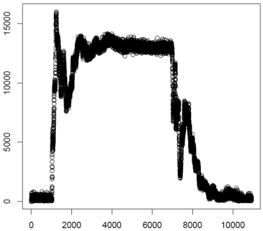
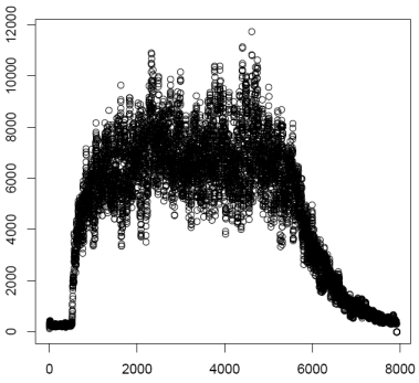
Once the two functions are defined the script will load in the file
"Pulse1k.txt" and rectify the data (take the absolute value).
Next the smoothing function is called and the data is down sampled by
44.1 times.
Since the sound file is sampled at 44.1 kHz, this down sampling makes
the time increment between adjacent data points equal to 1
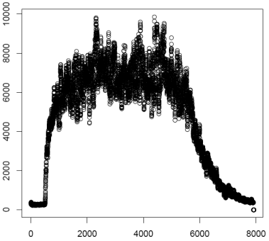
millisecond. Next this data is plotted and saved as the file
"Envelope1k.pdf". At this point the threshold function is used to
find the regions of acoustic energy growth and decay. The growth
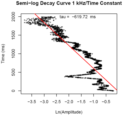
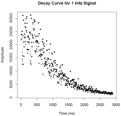
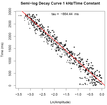
curve is plotted and saved as "GrowthCurve1k.pdf". Using a model
of exponential growth to a limit, the growth curve is transformed into
a linear relationship between time and transformed data. The
slope of this line is the time constant of this curve. Again this
linear relationship is plotted and saved as "GrowthFit1k.pdf". In
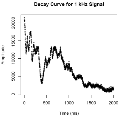
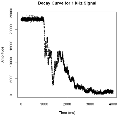
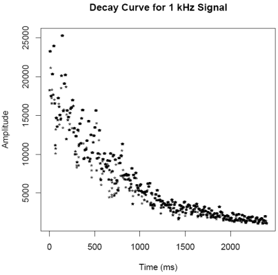
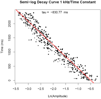
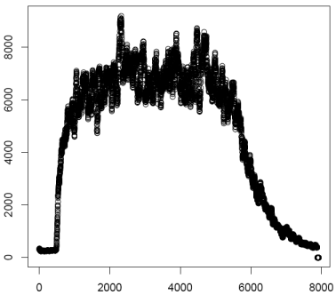
like fashion the decay curve is saved as "DecayCurve1k.pdf" and the
transformed data is saved as "DecayFit1k.pdf". Noise in the
collected data and the effect of standing waves in the room, can throw
the threshold detection calculation off. As a result, the last
part of the R-script allows a specific segment of the data to be
plotted and transformed. These results are also saved as
"DecayCurve1k.pdf" and "DecayFit1k.pdf" respectively. The
starting location of the decay curve will be around 5500 ms (5.5 s) and
end around 8000 ms (8.0 s).
The R-scripts for analyzing the pure tones was adjusted depending on
the frequency being analyzed. Since a 1kHz pure tone repeats
every 1 millisecond, setting the smoothing window to 44.1 samples
should effectively smooth out a constant amplitude tone. Since
the recorded data is rectified before smoothing, the rectified peaks
occur every 22.05 samples. Therefore, setting the smoothing
window to 23 samples gives fairly smooth data once the room reaches
equilibrium with respect to acoustic energy. At 500 Hz the
rectified data repeats every 44.1 samples, so a smoothing window of 45
data points is used. Similar adjustments are made for the
analysis of the 2 kHz and 4 kHz analysis. The following are the
R-scripts for those analyzes.
Links to
relevant R-scripts for analyzing room response to pure tones
Links to
relevant R-scripts for analyzing room response to warble and white noise
| 500 Hz |
1 kHz |
2 kHz |
4 kHz |
|
| Pure Tone |
0.664
± 0.013 s |
0.587 ± 0.008 s | 0.649 ± 0.009 s | 0.306 ± 0.006 s |
| Warble |
0.842 ± 0.008 s | 0.847 ± 0.006 s | 0.672 ± 0.005 s | 0.393 ± 0.007 s |
| White Noise |
0.827 ± 0.016 s | 0.813 ± 0.004 s | 0.653 ± 0.002 s | 0.374 ± 0.006 s |
| 500 Hz |
1 kHz |
2 kHz |
4 kHz |
|
| RT |
5.71 s |
5.61 s |
4.51 s |
2.58 s |